An Introduction to Automated Market Makers

Automated Market Makers (AMM’s) provide a simple mechanism for users of DeFi platforms to trade assets and provide liquidity. In this article, I will cover how these mechanisms work, the economics that back them, and some of the subtleties of their operation.
Background Info
In a prior article we discussed order books and how they are a mechanism that allows two parties to trade a pair of assets. We also discussed the concept of liquidity and how it represents how much of an asset is available to be bought or sold for a given price.
All exchanges (whether they be centralised or distributed) wish to have high liquidity so as to guarantee good prices to participants, and to reduce slippage. In order to facilitate this, most exchanges will have participants who take the role of market makers. A market maker is a participant who’s main goal is to provide liquidity, and quote on both sides of the book to facilitate this.
Market makers are commonly found on centralised exchanges. Such exchanges will provide API access so that these participants can easily connect to the exchange, and use sophisticated programs to quote for various products or pairs. Market making can be quite complex, and often involves changing your quotes rapidly when reacting to market movements, and other conditions. As such, to make a market on a regular order book requires the market maker to make a lot of rapid updates (100’s per second in some cases) in order to keep up.
gm crypto twitter
— ryuzaki (@0xRyuzaki) September 13, 2021
thought I'd kick things off by dropping some knowledge on electronic market making
a thread on how institutions are built by programming computers to buy low sell high
A History Of Automated Market Makers
Centralised exchanges have, well… centralised infrastructure, and therefore are able to support such high order throughput. In the world of DeFi (Decentralised Finance) however, everything is done on chain meaning that all instructions such as orders, amends, cancels etc. would need to be sent to and written to the blockchain. Around the time when DeFi was getting started (~2018), Ethereum was the chain of choice for such endeavours, due to its relatively high throughput and broad support for smart contracts.
At the time of writing, Ethereum can do roughly 10-30 transactions per second. Each transaction also has a non-negligible cost, with current gas prices sitting at around $50 each. Given those constraints, trying to use and maintain an order book would be problematic and likely not economically viable. What was needed was a trading mechanism that would provide the functionality to swap one asset for another at a fair price, but that (crucially) would not require constant fiddly and expensive adjustment like an order book.
In 2016, Ethereum creator Vitalik Buterin wrote a post on Reddit detailing an idea for a type of “decentralised exchange”. In it, he laid out a design for what would eventually become an Automated Market Maker. A smart contract that when invoked, would allow the swapping of one asset for another for a price determined by a mathematical relationship representing the supply/demand for the given assets.
One of the first DEXs to launch was Uniswap, which allowed anyone with ERC20 tokens to launch an AMM to swap any two tokens for each other. At the time of writing it is the DEX with the highest volume, and has spawned many competitors. AMM’s are a feature of almost all DEXs, and many different variants exist to satisfy different financial needs.
Economics of AMMs
While the motivation for creating AMMs was likely technology constraints, AMMs are essentially a distillation of the financial concept of supply and demand. Intuitively, if something is in high demand, but has limited supply, we would expect the price to be high. Likewise, if there is a glut of supply and no demand we would expect the price to be low.
With order books, this concept is encoded in the idea of impact prices. The less liquidity there is, the more it will cost to buy/sell an asset due to the fact that progressively higher/lower passive orders will need to be hit in order to fully fill an aggressive order. AMMs do not have such a luxury, but instead, they rely on a mathematical formula in order to model this concept.
Liquidity Pools
A liquidity pool is a smart contract structure that holds a certain quantity of tokens. The exact mechanics of what the pool does, or how it is deposited/credited varies depending on its purpose, however fundamentally it can be viewed as a bucket that contains some quantity of tokens

A visual representation of an Ethereum (ETH) and a Circle Stable USD (USDC) pool.
An AMM typically consists of two of these pools, backing the currency pair that the AMM represents. For instance, on a regular centralised exchange, we might see a trading pair e.g. ETH/USDC. This means that you can either:
- Buy ETH by selling your USDC.
- Sell ETH and receive (buy) USDC.
The liquidity to carry out these trades comes from the order book, where passive orders are placed to either buy or sell the pair at a price designated by the limit price of the order. In an AMM, this bid/ask liquidity comes from the two pools that back the trading pair. In this case, there is a pool of USDC and a pool of ETH available.
Constant Product AMMs
As mentioned, AMMs model price based on a mathematical formula instead of using order book price levels. There are many different formulas (we will cover these later), but for now we will focus on the most ubiquitous, which is the constant product AMM.
Right now, we have a pool of two tokens, but there is nothing that binds them together. When looking at the exchange rate between two tokens, we can note that the price is really a representation of the ratio of value between the two tokens. For instance, if the current price of ETH/USDC is 4,000 then that means that one ETH is worth 4,000 USDC. Conversely, one USDC is worth $ \frac{1}{4000} = 0.00025$ ETH. When dealing with AMMs, it is important to think of these price in terms of the ratio of “value” of one token to another.
Adding and removing liquidity from the pools is a separate topic that will be covered later, but for now we will assume that the liquidity pools start with an equal number of tokens in them. Every pool is governed by an equation. In the case of a constant product AMM the equation is:
$$ x \times y = k$$
Where $x$ and $y$ are the amounts of each of the two tokens, and $k$ is a constant. Depending on how much liquidity has been deposited into the pool (more on this later) this equation always holds. Consider the example below:

An initial setup of a constant product AMM
There 5 tokens deposited in each of the ETH and USDC pools. Therefore, the constant $k$ is always equal to $5 \times 5 = 25$ with this initial setup. This relationship is controlled by the smart contract that controls this particular (ETH/USDC) AMM. All interactions with the pools are therefore mediated and guarded by this contract.
Trading in an AMM
Right now we have an AMM set up with initial deposits on both sides of 5 ETH and 5 USDC respectively. The balance of these two tokens is very important, since this is what represents the price of the two assets. The ratio between the quantity of liquidity is what we can use to derive the (implied) price of each of the tokens in the other. To get the price of a token given a pool with tokens $x$ and $y$ we can use the following equations:
$$ P_x = \frac{Q_y}{Q_x} \text{ and } P_y = \frac{Q_x}{Q_y} $$
Where $P_{x/y}$ is the price of x/y, and $Q_{x/y}$ is the quantity of tokens in the liquidity pool of x/y. Right now, our pools both have the same quantity of tokens, so what we can deduce from this is that right now the price of ETH in USDC is 1, and likewise the price of USDC in ETH is 1. They are both equal to each other!
Buying
Let’s say that we want to buy 1 ETH. Thinking ahead, you might assume that the AMM would have the following idea:
Currently, my tokens are both equal in value. If someone wants one of my ETH, I should charge them 1 USDC because that is the fair price.
However, consider what would happen in that case. We would give the AMM 1 USDC and the AMM would put it in its USDC pool. It would then take 1 ETH from its ETH pool and give it to us. We have bought our 1 ETH, and the liquidity pool now has:
| Token | Balance |
|---|---|
| ETH | 4 |
| USDC | 6 |
All seems fine, but wait! We mentioned previously that the constant product equation must be satisfied at all times. So in this case, the quantity of ETH and USDC in the pools when multiplied must equal to the original value of 25. One thing to always keep in mind is that $k$ never changes during trades. This is important to understand, as early on this fact tripped me up frequently. As we will see later, $k$ only changes with deposits or withdrawals to the pool, not trades. What is $k$ right now?
$$ 4 \times 6 = 24 $$
So our AMM would not be allowed to do the above. What would it really do? Remember, the equation must always be maintained. That means that if we want to give away 1 ETH, we must charge more USDC. We can derive this amount by putting this all together into the following equation:
$$ (Q_{ETH} + \Delta Q_{ETH}) \times (Q_{USDC} + \Delta Q_{USDC}) = k $$
Where $Q_{x}$ and $\Delta Q_{x}$ represent the original quantity of token $x$, and the proposed change (trade amount) respectively. We already know the original quantities, and we know that $\Delta Q_{ETH}$ is -1 because we want to take 1 ETH from the pool. We can therefore re-arrange and get the following formula for the number of tokens that the AMM would take for such a trade:
$$ \Delta Q_{USDC} = \frac{k}{Q_{ETH} + \Delta Q_{ETH}} - Q_{USDC} $$
Plugging in our numbers we get $\frac{25}{5 - 1} - 5 = 6.25 - 5 = 1.25$. So the AMM must charge 1.25 USDC to buy 1 ETH. So now our AMM looks like this:

AMM state after a 1 ETH buy
Notice that the constant product equation is still maintained, since $4 \times 6.25 = 25$. The average price of the 1 ETH ended up being 1.25 USDC, even though initially the AMM’s current price was 1 to 1. Consider that we come in, and want to buy another 1 ETH from the pool. What happens this time? Reusing our formula from before: $\frac{25}{4 - 1} - 6.25 = 8.333 - 6.25 = 2.083$. So the next ETH that we bought cost ~2.083 USDC. Our AMM now looks like this:

AMM state after a subsequent 1 ETH buy
We could keep going. Buying another ETH would have cost us ~4.166 USDC. Notice three things happened when we continued buying ETH:
- The amount of ETH in the ETH pool decreased.
- The amount of USDC in the USDC pool increased.
- The price of each subsequent ETH bought increased as we kept buying.
In this way, as the supply of ETH decreases (amount in pool goes down), the price of ETH goes up as we would (economically) expect it to.
Selling
Say that we see our AMM in it’s final state from above with 3 ETH and 8.333 USDC, and a constant $k$ of 25. We decide we want to buy USDC by selling ETH. Say we want to sell 2 ETH, how much USDC would we get? We can use the formula again. This time our $\Delta Q_{ETH}$ is +2, because we will give the pool 2 ETH in exchange for some USDC. $\frac{25}{3 + 2} - 8.333 = 5 - 8.333 = -3.333$. In other words, the pool must lose (pay out as it is negative) 3.333 USDC for the 2 ETH.
So selling the 2 ETH on average netted us a price of 1.666 USD per ETH. Note that economically this also makes sense, since the original price the AMM was representing was $8.333 / 3 = 2.777$ USDC per ETH. Our pool is now back to where it started. There are 5 ETH and 5 USDC in the pools, and our constant remains 25. If we wanted to sell another 2 ETH, then the price would end up being: $\frac{25}{5 + 2} - 5 = 3.57 - 5 = -1.429$. That’s $\frac{1.429}{2} \approx 0.715$ USDC per ETH. So as before, we would continue getting a worse and worse (lower) price the more we sold.
Price vs Liquidity
A chart that is commonly used to illustrate the relationship between the liquidity of the pools, and the price of the token is the price impact chart showing how the liquidity of one pool changes with respect to the liquidity of the other pool.

Chart showing liquidity of USDC pool vs liquidity of ETH pool, assuming $Q_{ETH} = Q_{USDC} = 10$, and a constant $k$ of 100. This takes the form of a hyperbola.
Notice that you can draw two lines (as shown in the diagram above) to see how much of each token you would need to carry out the trade. The gradient of between these two points represents the average price for such a trade.
Slippage
In an earlier article we discussed how market orders can result in a worse average price outcome due to the distribution of liquidity in the order book. This effect is commonly known as slippage. In an AMM all orders are essentally market orders since there is no concept of discrete liquidity at different price levels. We also saw in the case where we bought 1 ETH from the initial equal price market maker that even though the current price was 1 to 1, we actually ended up paying 1.25 USDC. Therefore we could say that the extra 0.25 USDC was “slippage” from the 1 USDC we expected.
Slippage can be a risk since when we send the trade request, we can’t be certain of what price we might get. In order to mitigate this risk, AMMs typically come with a slippage tolerance setting. This is in some ways similar to a limit order seen in regular order books.
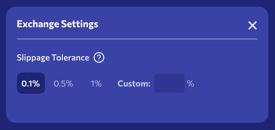
Slippage tolerance setting on the Orca DEX
Slippage is calculated as the percentage difference in the average price achieved, vs. the current prevailing price of the AMM. For instance, consider an AMM that has 100 ETH, 400,000 USDC, and a constant $k$ of $100 * 400,000 = 40,000,000$. This implies a prevailing price of $\frac{400,000}{100} = 4,000$ USDC per ETH. If we want to buy 1 ETH, that will end up costing us $\frac{40,000,000}{100 - 1} - 400,000 = 4040.4$ USDC. We can calculate slippage using the following formula:
$$ \%Slippage = 100 \times (\frac{Price_{achieved}}{Price_{expected}} - 1) $$
That implies a slippage of $100 \times (\frac{4,040.4}{4,000} - 1) \approx 1.01\%$. If we had set our slippage tolerance to 2% this trade would go through, as it implies we are comfortable with such a price. However, if our tolerance was set lower (say 0.5%) then this trade would be rejected to protect us from getting a worse price than we were comfortable with.
Slippage vs Liquidity
You might be aware that when using order books, the best way to reduce slippage is to make sure there is sufficient liquidity to absorb large market orders. This is after all what market makers are supposed to be doing. How does this work with AMMs? Consider the following AMMs for the same ETH/USDC pair, which both have an implied 1 to 1 price.

Two AMMs each with equal liquidity in both pools. A has 100 tokens in each pool, while B has 10,000 in each pool.
If we wanted to buy a certain amount of ETH from each of these pools, what would our slippage look like? The following table outlines how the price and slippage would behave:
| ETH Buy Qty | Price USDC (A) | Price USDC (B) | % Slippage (A) | % Slippage (B) |
|---|---|---|---|---|
| 1 | 1.0101 | 1.0001 | 1.0101 | 0.010001 |
| 5 | 1.05263 | 1.0005 | 5.26316 | 0.050025 |
| 10 | 1.11111 | 1.001 | 11.1111 | 0.1001 |
| 20 | 1.25 | 1.002 | 25 | 0.200401 |
Notice how dramatic the slippage difference is in the higher liquidity pool (B). Buying 20 ETH in B will give us just 0.2% slippage, while in the lower liquidity pool (A) it would cost us 25% more! This highlights how important liquidity is to a pool. A lower liquidity pool is just not an appealing trading venue for those clients wanting to transact there.
Adding Liquidity
We’ve discussed how we can trade tokens by taking/removing tokens from the two liquidity pools in the correct proportions to satisfy the equation governing the AMM. But notice that no matter how much we trade, the constant $k$ never changes. So how do the tokens get into the pool in the first place?
As well as trading, pools have the option to add liquidity. When the pool is first created, the creator of the pool must provide the initial liquidity for the two tokens in the pool. Uniquely, the creator is able to set the initial balances of the two pools according to how they see fit. It is of course in their interest to make sure that the proportion of tokens that they put in are in line with the current market price of the two tokens. Otherwise, they are exposed to being arbitraged (more on this later).
Say that the current ETH/USDC spot rate on centralised exchanges is \$4,000. The creator of an ETH/USDC AMM on a DEX will want to deposit 4,000 USDC into the USDC pool for each ETH that they deposit into the ETH pool. After this, other users are free to add liquidity to the pool. However, unlike the creator, they must deposit liquidity in the same proportion as the current balances. If the ETH/USD AMM has a current proportion of 1 ETH to 3,500 USDC then any new deposits must also be in this proportion. So if the user wants to deposit 10 ETH, they will also have to deposit 35,000 USDC at the same time.
Any user that provides liquidity to the pool is called a Liquidity Provider or LP. When a user deposits provides liquidity to the pool, typically they will be issued with something called Liquidity Provider Tokens or LP Tokens. The amount of tokens issued, is dependent on the amount of liquidity provided. For a constant product AMM this amount is:
$$ \Delta Q_{LP} = Q_{LP} \times \frac{\Delta Q_{x}}{Q_{x}} $$
Where $Q_{LP/x}$ are the totals of the liquidity tokens and deposit tokens present respectively, and $\Delta Q_{LP/x}$ are the changes in those tokens. $x$ in this case is either of the token pair, and whichever results in the smaller amount of LP tokens issued is the one chosen. When an initial deposit is made by the person creating the pool, the total quantity in the pool and of the LP tokens is 0, making the above formula not viable. To work around this, UniSwap V2 sets the initial amount of tokens to the geometric mean of the two tokens deposited.
$$ Q_{LP} = \sqrt{Q_{x} \times Q_{y}} $$
The LP tokens represent the proportion ownership of the pool as well as any fees that were collected. Each liquidity provider is entitled to their portion based on the amount of LP tokens they hold vs the total amount outstanding. Say that an initial LP provides 10 ETH and 40,000 USDC to a pool. They would receive $\sqrt{10 \times 40,000} \approx 632.46$ LP tokens for their initial liquidity. Later, another LP joins the pool and deposits a further 5 ETH, and 20,000 USDC (as they must be in proportion). They receive $632.46 \times \frac{5}{10} = 316.23$ LP tokens for their additional liquidity.
Notice that given that the second LP provided half the liquidity of the first LP, we would expect them to receive one third of the total assets and fees of the AMM. Comparing LP tokens, the first LP will receive $\frac{316.23}{632.46 + 316.23} \approx 0.333$ which is one third, as we expected. One important thing to note is that adding and removing liquidity is the only way for the $k$ constant to change. After the first deposit, $k$ was $10 \times 40,000 = 400,000$. After the second deposit, $k$ was $15 \times 60,000 = 900,000$. As always however, $k$ must represent the product of the quantities in the two underlying pools.
For an in depth look at LP tokens (and other concepts) I highly recommend this series by Anton Kuznetsov, which shows you how to build an AMM from scratch in Solidity.
Correction: Previously it was incorrectly stated here that the geometric mean formula was used for new deposits, when in fact it is only used for initial deposits. Thanks to @latte_jed for pointing it out to me.
Removing Liquidity
Just as liquidity can be added into an AMM, liquidity can also be removed at the discretion of the liquidity provider. The share of LP tokens that they hold will entitle them to withdraw their portion of the assets in the two pools, but also any fees that have accumulated as a result of trading. Say that an LP holds 10% of the LP tokens of a ETH/USDC AMM that currently holds 100 ETH and 350,000 USDC. The user can burn their LP tokens (essentially discard them), and receive 10% of the pool.
The user will always receive assets in the correct proportions. As such, if the above client were to burn all of their LP tokens they would receive 10 ETH, and 35,000 USDC. Due to the decrease in total LP tokens, the ownership percentage of the pool for the other 90% of the LPs has increased, though in terms of value they still own the same amount. If any fees were accrued while the user held the LP tokens, these would also get paid out as part of the withdrawal process.
As before, the $k$ constant has now also reduced. It was initially $100 \times 350,000 = 35,000,000$. As a result of the withdrawal $k$ is now $90 \times 315,000 = 28,350,000$.
Fees
One of the appeals of being a liquidity provider is that anyone can be a market maker, but without the hideously complex technology setup that is required to be one on a traditional order book. All one needs to do is provide the required tokens in the required ratio, and sit back and collect the fees (it turns out it is more complicated than that, as we will find out later).
Each AMM will have some sort of fee structure in place, which will reward LPs for their liquidity. For instance, on UniSwap the most common fee amount is 0.3%. This means that for any trade, 0.3% of the value of the trade (for both tokens) will be left in the pool, and be (proportionally) assigned to the LPs. That means someone selling 1 ETH for 4,000 USDC would actually receive $0.997 \times 4,000 = 3,988$ USDC. That means that they paid a fee of 12 USDC for the trade, and that 12 USDC would remain inside the USDC pool. Note, that these fees need to be included in the formulas in the previous section, since $k$ must still be maintained. For brevity however, this will not be included in this article, and is left as an exercise for the reader.
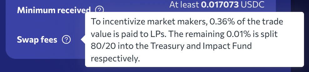
Breakdown of fees on the Orca DEX
Not all distributed exchanges work the same way, for instance Orca gives only a portion of the fees to LPs, while a smaller portion goes to a treasury fund which is typically a pool of money that is used for development and governance of the DEX itself.
Price Arbitrage
Order books have market makers that constantly adjust their bids and asks in order to keep in line with the rest of the market. Not doing so would be problematic for them, since that would allow other participants to take advantage of their mispriced orders. The reason for this is that if you manage to find an asset on one exchange that is being sold at a lower price than it is being bought on another exchange, you can use arbitrage to make the difference.
Arbitrage means doing something to make a risk free profit. Exchange arbitrage works because there are many different market makers and many different exchanges. Occasionally, the price of an asset on one exchange may drift away from the price on another exchange. Consider the following quotes for e.g. ETH/USDC:
| Exchange | Bid | Ask |
|---|---|---|
| Binance | 4,000 | 4,010 |
| FTX | 3,990 | 4,000 |
| Kraken | 3,980 | 3,990 |
Remember, you buy at the Ask, and sell at the Bid. Given that, notice that there is an arbitrage or arb opportunity between Kraken and Binance. To do this requires the following steps:
- Buy 1 ETH at 3,990 USDC on Kraken. You now have 1 ETH, and are down 3,990 USDC.
- Take the 1 ETH to Binance, and sell it for 4,000 USDC. You now have no ETH, and $4,000 - 3,990 = 10$ USDC.
Just buy buying and selling once you have made a (theoretically) risk free 10 USDC. Of course, it is rarely that simple, as there are a host of things to contend with.
- Fees
- Fees can be an issue, since they reduce your profit, and therefore make some arb opportunities not economically viable.
- Slippage
- Slippage can also make an arb unprofitable. Though the best bid/ask might seem tempting, you may find there is only e.g. \$100 worth of liquidity there, which is barely enough to make a profit (if any).
- Moving Funds
- Moving money between exchanges is time consuming, and not always free either. Normally you would need funds in many different places to be able to instantly execute an arbitrage opportunity. Having that much capital sitting around is expensive (it could be e.g. lent out for a guaranteed return instead).
- Latency
- It takes time for the message from the exchange to arrive at your computer, and for you to process it to identify the opportunity. Then you need to send an order which also takes time. You might find that by the time you do all of this, the opportunity is already gone, and you might even be left with a loss just for trying!
Arbitrage however is what makes sure that the different markets are kept in line, since even the slightest mispricing may lead to an arbitrage opportunity which will be quickly eaten away by bots. With AMMs, this mechanism is quite similar. Consider the following pools for ETH/USDC:
| Pool | Qty (ETH) | Qty (USDC) | Implied Price (USDC) |
|---|---|---|---|
| A | 100 | 400,000 | 4,000 |
| B | 100 | 390,000 | 3,900 |
In this case, an enterprising user could do the following:
- Buy 0.6 ETH on pool B, with slippage this would result in an approximate cost of 2,749.2 USDC using the earlier formulas.
- Take the 0.6 ETH, and sell it on pool A. This would yield 2,780.5 USDC, leaving the user with a profit of $2,780.5 - 2,749.2 \approx 31.3$ USDC.
After all of this, what do the above AMM’s look like?
| Pool | Qty (ETH) | Qty (USDC) | Implied Price (USDC) |
|---|---|---|---|
| A | 100.6 | 397,614.3 | 3,952.4 |
| B | 99.4 | 392,354.1 | 3,947.2 |
Notice that as a result of these trades, the price of the two AMMs has now (mostly) converged. Of course, this is ignoring fees and other similar things, however this basic mechanism is how traders can keep AMMs in line with the rest of the market, be it other AMMs or centralised exchanges (the principle is the same).
Astute readers may notice that there is still an arbitrage opportunity left, since the prices of the two AMMs have not fully converged. For those interested, the following GitHub page outlines the formula and derivation for finding the optimal arbitrage amount. In the above case, the optimal arbitrage amount would be $\approx 0.633$ ETH.
Impermanent Loss
A prudent rule to follow when assessing financial investments, is to always ask two questions:
- Where’s the money coming from?
- Where’s the risk?
If we treat being a liquidity provider as an investment, we know that the money comes from fees that users pay when trading. So far so good for point 1. But as for point 2, where exactly is the risk? Traditional market makers have all sorts of risks, such as e.g. inventory risk, which is the risk that they will end up holding too much of one asset, and that assets price moves against them. AMMs might seem like a fire and forget solution for passively generating returns on your liquidity, but there are indeed risks involved.
For a basic case, consider an AMM that has 5 ETH and 5 USDC. The liquidity provider set up this AMM with an equal value between the two, so their price is 1 to 1. The LP also got LP tokens from the AMM, representing 100% ownership of all of the assets inside, as well as any fees made by the AMM.
| Token | Balance |
|---|---|
| ETH | 5 |
| USDC | 5 |
Let’s say that a user comes in, and makes a trade to buy 1 ETH from the pool. According to the constant product formula they will pay 1.25 USDC. The pool now looks like this:
| Token | Balance |
|---|---|
| ETH | 4 |
| USDC | 6.25 |
The implied cost of ETH is now $\frac{6.25}{4} = 1.5625$ USDC. Let’s say that our liquidity provider decides to burn all of his LP tokens, and withdraw all of the liquidity in the AMM. After all, they are entitled to 100% of the liqudity. The LP ends up with 4 ETH and 6.25 USDC. Now let’s compare before and after:
The user originally started with 5 ETH and 5 USDC that they deposited into the pool. After withdrawing from the liquidity pool, the user now has 4 ETH and 6.25 USDC. Let’s calculate the value of the assets as they are now, vs. if the user had done nothing and just held onto the assets as they were. We will calculate the total portfolio value in USDC.
| Scenario | Amount ETH | Amount USDC | Current ETH/USD Price | Portfolio Value (USDC) |
|---|---|---|---|---|
| Do Nothing | 5 | 5 | 1.5625 | 12.8125 |
| Provide Liquidity | 4 | 6.25 | 1.5625 | 12.5 |
So essentially, if we had done nothing but just held, we would have been better off than providing liquidity in the AMM. We would have gained an additional $\approx 0.3$ USDC by not participating. This effect gets worse the larger the price difference. The following chart shows how this loss looks like given a price difference in the two tokens.

% impermanent loss as a function of % change in price between two tokens in an AMM
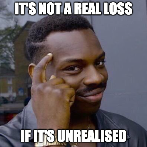
While the user keeps hold of the LP tokens, and does not withdraw their liquidity, this phenomenon is called impermanent loss. It is called impermanent, because much like “unrealised” loss, it is not a real loss until you withdraw liquidity. Of course, this fails to take into account that from a mark to market perspective, you have lost money. In fact, a study done by Bancor in Nov. 2021 showed that close to half of all liquidity providers had lost money due to impermanent loss.
Logically, it follows that you have the least chance of suffering an impermanent loss if:
- Fees are high enough that they cover any theoretical loss.
- The two tokens being traded are very highly correlated, and therefore will not fluctuate much against each other.
Stablecoins such as Tether, USDC, and DAI are all approximately pegged to the US dollar. Therefore, one assumes that they will move in tandem, and such pairs are popular on various DEXs for this reason. DEXs can also attract users to provide liquidity on high volatility pairs by increasing fees on that AMM. The idea is that given a high enough fee, almost any impermanent loss will be worth it since the fees will make up for it. In this way, it mirrors how highly volatile pairs on traditional order books have large spreads, since these are essentially a fee to the market maker for taking on the inventory risk on that pair.
Other AMM Flavours
In this article we have been discussing primarily the constant product AMM, and this is by far the most common. However, there are now many different variants that have sprung up. Below is a short and non-exhaustive list of some popular ones.
Constant Sum
This type of AMM is represented by the equation:
$$ x + y = k $$
They are also sometimes called constant price AMMs, due to the fact that this invariant causes the price to be the same (1) for whichever token is bought or sold. Such models can be useful for assets which are always meant to be traded 1 to 1, however they can run into issues since they do not adjust for supply and demand. For a more detailed look, I would suggest this article.
Constant Mean
A generalised version of the constant product AMM invented by Balancer. Each asset can have a different weighting. In general:
$$ \prod_{i}^{n}{Q_{i}^{w_{i}}} = k $$
Where $Q_{i}$ is the quantity of each asset, and ${w_i}$ is the weighting for each asset. For instance, if each asset is weighted the same, then the geometric mean of three assets would be $x^{\frac{1}{3}} \times y^{\frac{1}{3}} \times z^{\frac{1}{3}} = k$. Such AMMs are useful for more complex swaps where more than two assets have a relationship.
Stableswap
StableSwap is a type of AMM invented by Curve Finance. It can be called a hybrid AMM since it uses elements from both the constant product and constant sum market makers. StableSwap is primarily designed for trading stablecoins (coins pegged to a fiat currency), and has a different slippage profile compared to either of its predecessors.
The derivation of the equation is quite involved, however the below chart sumarises how the curve looks compared to the regular constant product or constant sum invariants. Notice how the price impact is mostly linear when there are small differences in liquidity, only increasing once the difference becomes large. Using this method, StableSwap aims to keep the price stable within certain liquidity ranges, and therefore reduce the cost of swapping stable coins, while still retaining the ability to react to extreneous supply/demand issues.
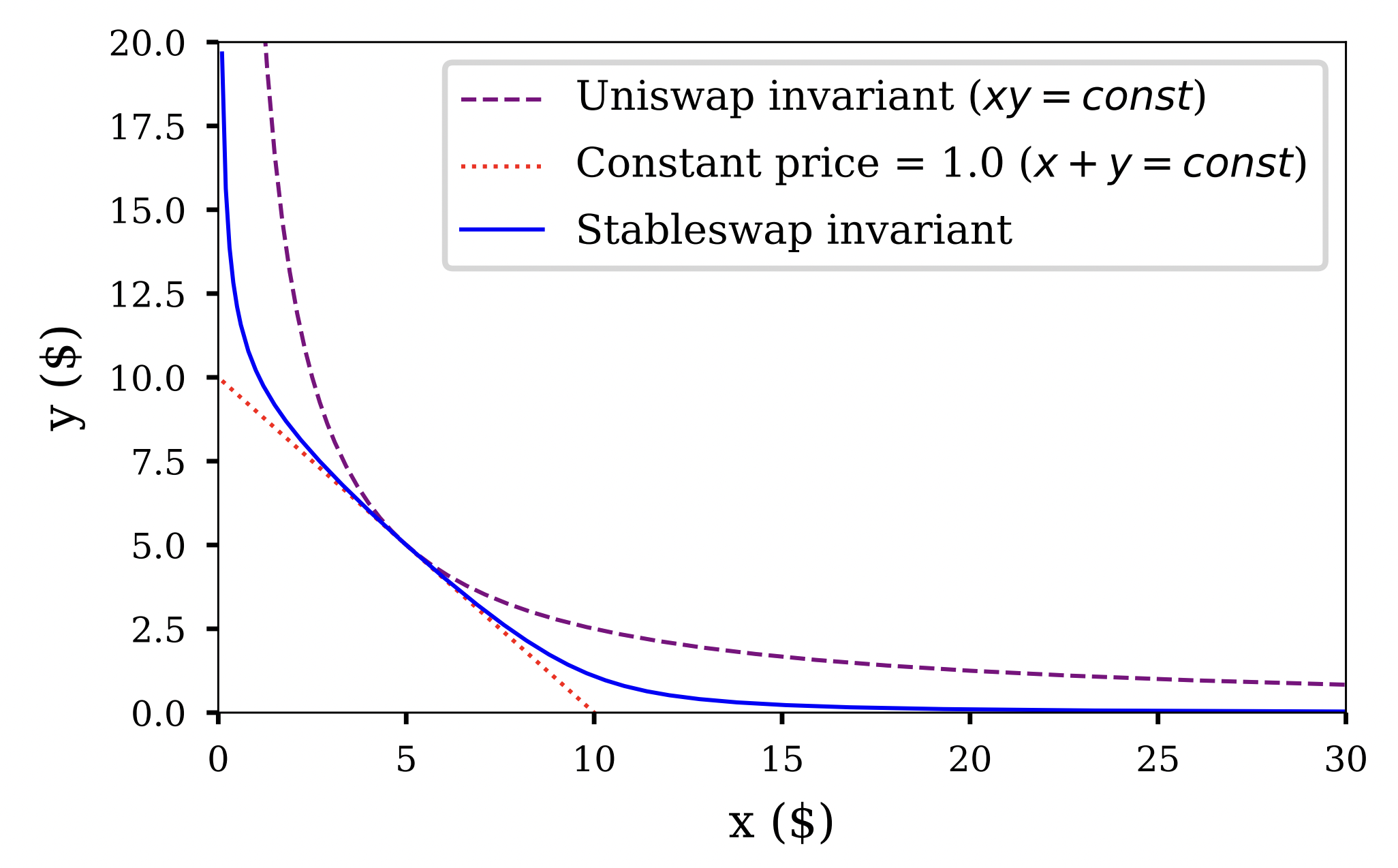
StableSwap slippage curve compared to a constant product (UniSwap) and a constant sum AMM. Source: StableSwap whitepaper
Equivalent Order Books
If a constant product AMM were to be represented as an order book, what would it look like? There are some differences. For instance, an AMM is a continuous function, while an order book due to its lot size and tick size has discrete liquidity. We can create a model of an order book if it was an AMM by analysing how the amount of notional required for each subsequent trade increases, and what price level and quantity would be required to fulfill that.
The following paper by @ProfessorJey is quite math heavy, but does outline the equations needed to represent this. In short, the equation for the cumulative quantity at any price be summarised as:
$$ Q_{cum}(p)=\begin{cases} \begin{aligned} \ & x_{0}(\sqrt{\frac{P_{0}}{P}} - 1) & \text{if } p < p_{0} \newline \ & 0 &\text{if } p = p_{0} \newline \ & x_{0}(1 - \sqrt{\frac{P_{0}}{P}}) & \text{if } p < p_{0} \end{aligned} \end{cases} $$
Where $Q_{cum}(p)$ is the cumulative quantity at any price (think of this like a depth chart), $p_{0}$ is the initial price of the AMM (mid price essentially), $p$ is the current price, and $x_{0}$ is the initial quantity of the base currency in the AMM. This leads to an order book with the following shape:
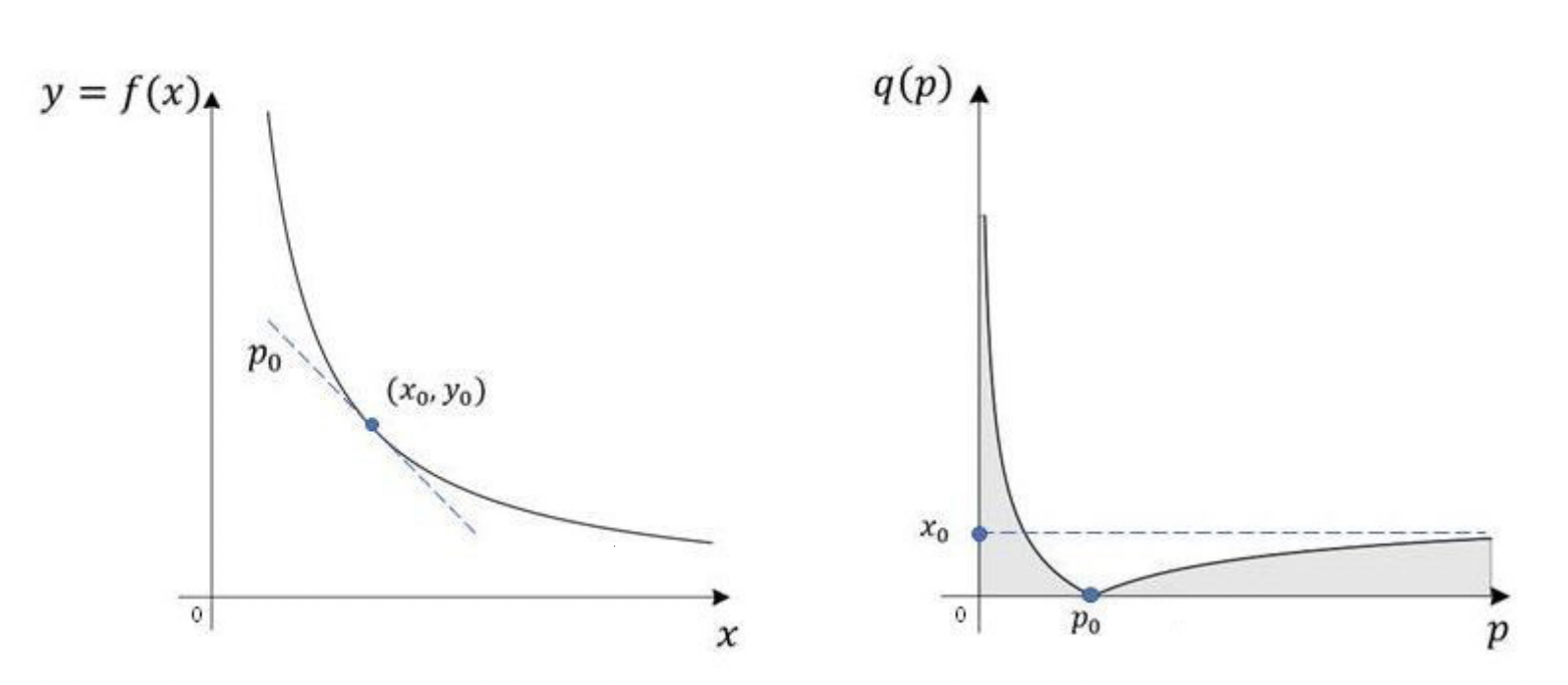
Constant product pricing curve (left) vs. equivalent order book (right). Source: J. Young, Oct. 2020, On Equivalence of Automated Market Maker and Limit Order Book Systems
We note that it fits our expectations. In order to keep buying in an AMM, we would start to receive higher and higher prices the more we bought. This corresponds to an infinite amount of small orders placed at increasingly higher and higher prices. The chart below shows what that might look like for an order book that has an order size of 0.01.

Theoretical distribution of small sell orders in an order book to have equivalent liquidity to an AMM with $x_{0} = y_{0} = k = 1$. Initial price $p_{0}$ is 1.
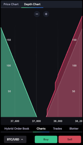
Real order books of course do not follow such a distribution perfectly, not least of which because it would require placing infinitesimally small orders somewhere near infinity. It would be interesting to do some research into how closely these two methods behave, however just glancing at FTX you can see that the shape of the cumulative liquidity does follow a similar pattern of high liquidity near the mid price, and increasingly lower liquidity and prices further from that.
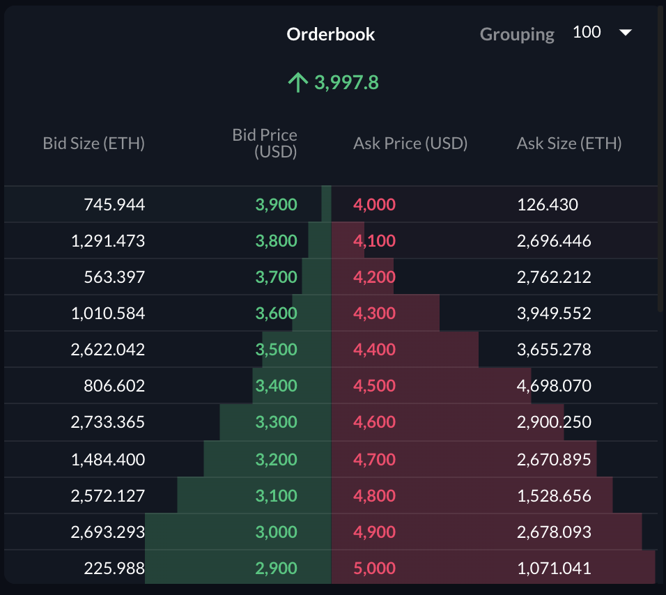
Snapshot of the cumulative book for ETH/USD on FTX.
Order books give traders much finer granularity control of their liquidity, meaning that they can adjust their liquidity profile much more finely. With AMM’s, increasingly complex formulas are required to match everyone’s requirements, which is not always possible. One definite benefit of AMMs however is their ease of use. Market making in an order book is a complex endeavour, and this means that retail clients are unable to participate. With AMMs, they can passively provide liquidity in exchange for fees.
This means that there is more liquidity available to the market, and less dependency on a handful of large market makers. However, the risk of impermanent loss means that clients wanting to place their funds in an AMM should consider carefully what their expected returns will be given the volatility of the tokens.
AMM / Order Book Hybrids
Recently, platforms are starting to spring up claiming to offer a “hybrid” solution between an AMM and an order book. Platforms such as Bullish and OneSwap claim to offer increased liquidity by allowing users to trade against BOTH an AMM and an order book. By doing this, they hope to be able to get the passive liquidity of the AMM as well as the more finely controlled liquidity of the professional market makers.
This technology is quite new, and there is limited information on it, however this post on ethresear.ch goes through some of the mathematics. The general idea is that order matching will query both a limit order book and an AMM for a certain price level. If the order book has the liquidity it is taken first. If there is further liquidity required to fill the order, the AMM is hit until the price movement moves to the next price level on the order book, and then the process repeats until the whole order is filled. It is an interesting combination of the discrete liquidity of the order book, and the continuous liquidity of the AMM.
Screenshot of the bullish.com “hybrid” AMM/Order Book. Notice the distribution seen in the previous diagram (zoomed in), with limit orders layered on top. Source: @kenny_lienhard
On-chain I think this is probably a viable idea. Newer, higher throughput chains such as Solana have made it possible to have an actual working order book on-chain, with slow, but workable performance. Projects such as Serum now use on-chain order books to provide a trading experience which is not drastically far off a centralised exchange, though with obviously much decreased performance and much lower volume. An interesting direction would be the combination of on-chain AMMs and centralised order books. This would provide much higher access to liqudity, however from a technical perspective I could see this being complex to coordinate.
Glossary
- Add Liquidity
- To add liquidity (tokens) to an AMM
- Arbitrage (Arb)
- To make a risk free profit buying one asset low, and selling it high somewhere else.
- Automated Market Maker (AMM)
- A smart contract that manages two or more liquidity pools and allows swapping of tokens according to a predetermined formula.
- Burn Tokens
- The action of destroying tokens. Used in the context of burning LP tokens to withdraw liquidity from an AMM.
- Constant Price AMM
- See Constant Sum AMM.
- Constant Product AMM
- The most common type of AMM. Accounts for supply/demand when swapping tokens.
- Constant Sum AMM
- A type of AMM that maintains a constant price between its tokens.
- Impermanent Loss
- A loss where the price between two tokens changes, and the liquidity in the pool becomes worth less than having held it as is.
- Liquidity Pool
- A smart contract representing a “bucket” of tokens.
- Liquidity Provider (LP)
- A user who deposits liquidity into an AMM.
- Liquidity Provider (LP) Tokens
- A special token that represents ownership of some liquidity in an AMM.
- On-Chain
- Activities carried out on the blockchain, rather than on a centralised system.
- Slippage
- The proportionate difference in average price for a trade between what was expected, and what was achieved.
- Slippage Tolerance
- A setting used by AMMs to prevent loss of funds due to excessive slippage on a trade.
- Smart Contract
- A type of program that runs on a blockchain.
- Treasury Fund
- A special fund controlled by a DEX that is used to manage and improve a DEX.